Category: Uncategorized

Normality is one of the most important assumptions in statistical analysis. Before running t-tests, ANOVA, regression, or any parametric test, you need to know whether your data follows a normal distribution. If it doesn’t, your results may be misleading – and any insights drawn from them, unreliable.

SPSS makes normality testing straightforward, but only if you know which tests to run, how to read the output, and what to do when your data fails the assumption.

This guide walks you through every step: the menu path, the tests to use, how to interpret the numbers, and how to handle non-normal data. It is written for researchers, analysts, and market research teams who need clean, defensible results to support faster decision-making.

Why Normality Testing Matters

Most parametric tests assume that your continuous variable is approximately normally distributed. When this assumption holds, your test results are accurate, and your conclusions are sound. When it fails, you risk:

• Inflated Type I or Type II errors
• Misleading confidence intervals
• Incorrect p-values
• Flawed business or research decisions

For organisations running large-scale studies, normality testing is not a checkbox. It is a quality gate. It protects the integrity of every analysis that follows and ensures the data feeding into reports, dashboards, and stakeholder presentations is fit for purpose.

In market research, where insights guide product launches, pricing strategy, and customer experience investments, getting this step right is non-negotiable.

What “Normal Distribution” Actually Means

A normal distribution is symmetrical and bell-shaped. The mean, median, and mode are roughly equal. Most values cluster around the centre, with fewer values appearing as you move toward the extremes.

In real-world datasets, perfect normality is rare. What you are testing for is whether your data is approximately normal – close enough that parametric tests will produce reliable results.

There are two ways to assess this in SPSS:

• Numerical methods – statistical tests that give you a clear yes or no
• Graphical methods – visual plots that show the shape of your data

Best practice is to use both. Numbers give you objectivity. Plots give you context.

Methods SPSS Provides for Testing Normality

SPSS offers several tools for normality assessment, all accessible through the Explore command:

Method	Type	Best For
Shapiro-Wilk Test	Numerical	Sample sizes under 2,000 (most reliable for n < 50)
Kolmogorov-Smirnov Test	Numerical	Larger samples, less sensitive than Shapiro-Wilk
Skewness & Kurtosis	Numerical	Quick descriptive check
Histogram	Graphical	Visual shape assessment
Normal Q-Q Plot	Graphical	Comparing data to a theoretical normal distribution
Box Plot	Graphical	Spotting outliers and symmetry

The Shapiro-Wilk test is the most widely recommended numerical test. It is sensitive and works well across most sample sizes you will encounter in research projects.

Step-by-Step: Testing Normality in SPSS

Here is the full procedure using the Explore command. This works in SPSS versions 17 through 30, including the subscription version.

Step 1: Open the Explore Dialogue

From the top menu, click: Analyze → Descriptive Statistics → Explore…

This opens the Explore dialogue box.

Step 2: Move Your Variable into the Dependent List

Select the continuous variable you want to test for normality. Move it into the Dependent List box using the arrow button or drag-and-drop.

If you want to test normality across groups – for example, comparing male and female respondents – move your categorical grouping variable into the Factor List box. SPSS will then test normality for each group separately.

Step 3: Configure the Plots

Click the Plots… button. In the dialogue that opens:

• Tick Histogram
• Keep Stem-and-leaf ticked
• Tick Normality plots with tests

This single setting unlocks the Shapiro-Wilk and Kolmogorov-Smirnov tests along with the Q-Q plot.

Step 4: Run the Analysis

Click Continue, then click OK in the main Explore dialogue.

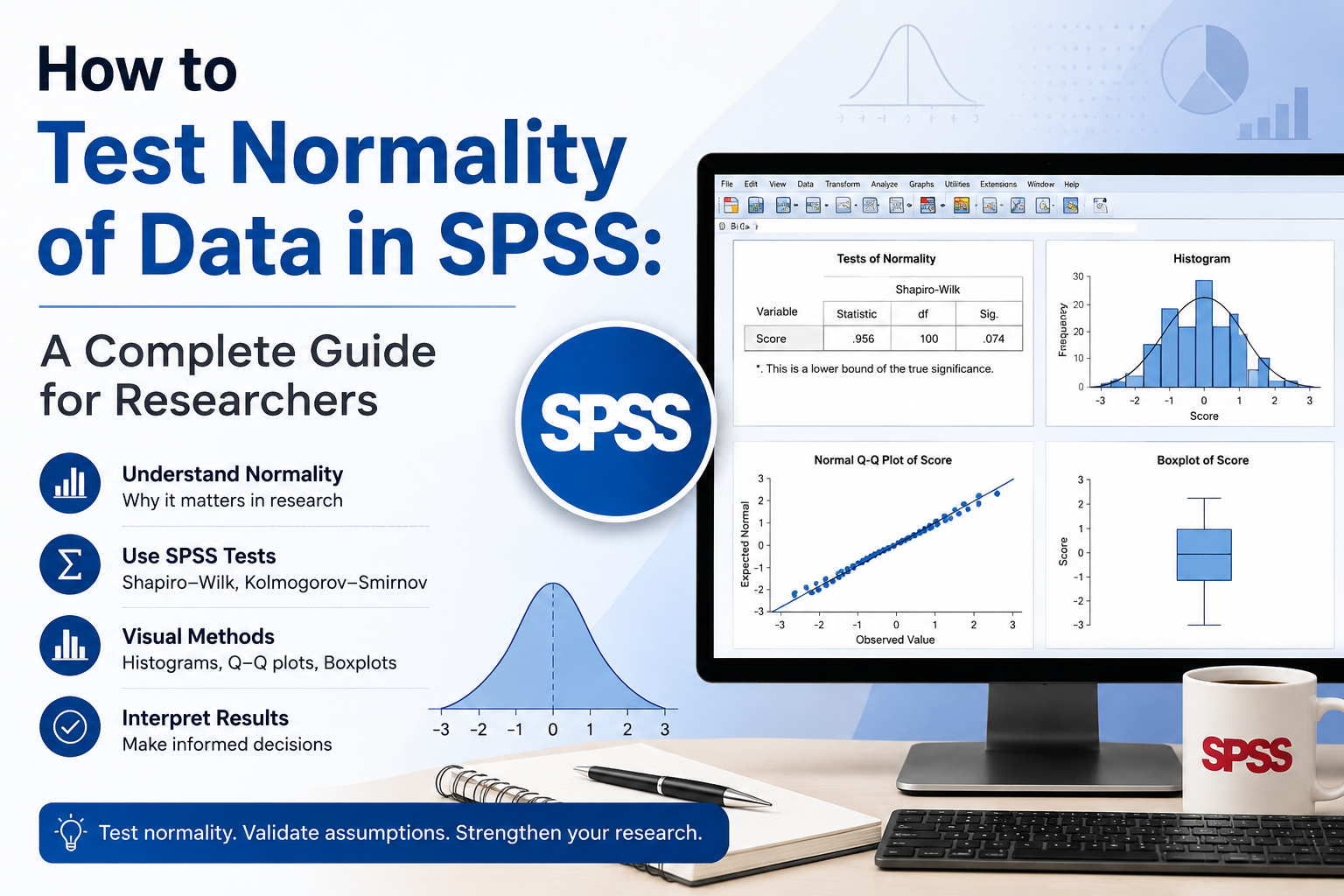
SPSS will generate a full output including descriptive statistics, the Tests of Normality table, histograms, stem-and-leaf plots, Q-Q plots, detrended Q-Q plots, and box plots.

Reading the SPSS Output

The output looks dense at first. Focus on these key sections.

The Tests of Normality Table

This is the heart of your numerical assessment. Look at the Sig. (p-value) column under Shapiro-Wilk.

• p > 0.05 → Data does not significantly deviate from normality. Assumption is met.
• p < 0.05 → Data significantly deviates from normality. Assumption is violated.

Note the logic carefully. A high p-value is good news. It means there is no significant difference between your data and a normal distribution.

Skewness and Kurtosis

In the Descriptives table, check the skewness and kurtosis values.

• Skewness measures asymmetry. Acceptable range: -1 to +1.
• Kurtosis measures the peakedness of the distribution. Acceptable range: -1 to +1.

You can also calculate z-scores by dividing each value by its standard error. Z-scores between -1.96 and +1.96 indicate acceptable normality at the 0.05 level.

Histogram

Look for a roughly symmetrical, bell-shaped curve. Double-click the histogram in SPSS to open the Chart Editor, then add a distribution curve to make symmetry easier to judge.

Normal Q-Q Plot

In a Q-Q plot, your data points are compared to a theoretical normal distribution. If the points lie close to the diagonal line, your data is approximately normal. Significant departures from the line – curves, S-shapes, or scattered points – suggest non-normality.

Box Plot

A symmetrical box, whiskers of similar length, and no outliers suggest normality. Heavy tails or visible outliers may indicate problems.

A Worked Example

Imagine a market research dataset measuring customer satisfaction scores for 80 respondents in a brand-tracking study. You run the Explore procedure and get the following:

• Mean: 22.01
• Median: 22.00
• Skewness: 0.049 (well within -1 to +1)
• Kurtosis: -0.442 (within -1 to +1)
• Shapiro-Wilk p-value: 0.585

The histogram is roughly symmetrical. Points on the Q-Q plot sit close to the diagonal line. The box plot is symmetric with no outliers.

Conclusion: The variable is approximately normally distributed. You can proceed with parametric tests.

This is the kind of clean, defensible result every research team wants. When all indicators agree, the decision is clear. When they disagree, you need to make a judgment call.

What to Do When Indicators Disagree

Sometimes the Shapiro-Wilk test says one thing and the histogram suggests another. This is common with large samples. The Shapiro-Wilk test becomes very sensitive at high n – it can flag trivial deviations as statistically significant.

Use this decision framework:

• Small sample (n < 50): Rely more heavily on the Shapiro-Wilk test.
• Medium sample (50–300): Combine Shapiro-Wilk with skewness, kurtosis, and visual plots.
• Large sample (n > 300): Trust visual methods more. The Central Limit Theorem also means many parametric tests are robust to mild non-normality at this scale.

For high-stakes research, document your reasoning. State which methods you used, what they showed, and why you made the call you did. This transparency strengthens the credibility of your findings.

Testing Normality Across Groups

In many studies, you need normality within each group of a categorical variable – not just the overall sample. For example, testing whether income is normally distributed for both urban and rural respondents before running a t-test.

The procedure is the same:

1. Analyze → Descriptive Statistics → Explore…
2. Move your continuous variable into the Dependent List
3. Move your grouping variable into the Factor List
4. Configure plots as before
5. Click OK

SPSS will produce separate statistics and graphs for each group. You may find that data is normal in one group and not the other. This is important information for choosing your next test.

What If Your Data Fails the Normality Test?

A failed normality test is not the end of your analysis. You have several options.

1. Transform the Variable

Common transformations include:

• Logarithmic transformation for right-skewed data
• Square root transformation for moderately skewed data
• Inverse transformation for severely skewed data
• Reflect-and-transform for left-skewed data

In SPSS, use Transform → Compute Variable… to create a new variable. Then retest the transformed variable for normality.

2. Use Non-Parametric Tests

If transformation does not help, switch to a non-parametric equivalent:

• Mann-Whitney U instead of an independent samples t-test
• Wilcoxon signed-rank instead of a paired t-test
• Kruskal-Wallis instead of one-way ANOVA
• Spearman’s correlation instead of Pearson’s

Non-parametric tests do not assume normality. They are less powerful but more robust.

3. Rely on the Central Limit Theorem

For large samples, parametric tests are remarkably robust to non-normality. If n is large enough – typically over 30 per group, often more – mild violations of normality may not meaningfully affect your results.

4. Investigate Outliers

Sometimes non-normality is caused by a handful of extreme values. Examine your data for entry errors, measurement issues, or genuine anomalies. Removing or correcting outliers – with proper justification – can restore normality.

Common Mistakes to Avoid

Even experienced analysts slip up here. Watch for these pitfalls:

• Treating p > 0.05 as “proof” of normality. It only means you cannot reject normality. The data may still deviate in ways that matter.
• Ignoring sample size effects. A statistically significant Shapiro-Wilk result with n = 5,000 may reflect a trivial real-world deviation.
• Relying on one method only. Numerical tests can be over- or undersensitive. Always pair them with visual inspection.
• Skipping group-level testing. Overall normality does not guarantee normality within subgroups.
• Forgetting to retest after transformation. A transformed variable must be retested to confirm the fix worked.

When Normality Testing Is Part of a Larger Workflow

In modern research operations, normality testing rarely happens in isolation. It sits inside a broader pipeline: data collection, cleaning, validation, analysis, reporting, and dashboarding. Each stage feeds the next, and a weak assumption check early on can compromise everything downstream.

For research teams running multiple concurrent projects across geographies and data sources, the challenge is scale. Manual assumption checks slow projects down. Automated, repeatable workflows – built around SPSS, R, Python, or integrated platforms – protect data quality without bottlenecking timelines.

This is where modern research infrastructure makes a difference. Standardised assumption testing, audit trails, real-time dashboards, and secure data handling turn statistical rigour from a friction point into a foundation for faster, more confident decisions.

Final Checklist Before Running Parametric Tests

Before moving on to your main analysis, confirm:

• You ran the Explore procedure with normality plots and tests enabled
• The Shapiro-Wilk p-value is above 0.05 (or sample-size-adjusted judgment applies)
• Skewness and kurtosis values fall within acceptable ranges
• The histogram and Q-Q plot visually support normality
• You tested normality within each group, where relevant
• You documented the test results and your interpretation

Once these are in place, you can confidently proceed with parametric analysis – and trust the insights that follow.

Closing Thought

Normality testing in SPSS is simple in execution but consequential in impact. Done well, it strengthens every statistical conclusion you draw. Done poorly, or skipped entirely, it undermines them.

For organisations where research drives strategy – market intelligence, customer insights, healthcare studies, social research – the difference between a defensible result and a questionable one often comes down to how well the early assumption checks were handled.

At Linkinfotech, we work alongside research teams to build scalable, technology-driven research operations where data quality, statistical rigour, and faster decision-making come standard. From survey programming to advanced analytics, our infrastructure ensures every analysis rests on a foundation you can trust.

If you would like to talk through how robust normality testing fits into your wider research operations. Get in touch.

In any market research project, the quality of your analysis depends on something most teams overlook: how variables are defined before a single test is run.

SPSS is one of the most widely used statistical platforms in research operations, and it has very specific rules about how it treats data. Get the variable type wrong, and your descriptive statistics, regressions, and dashboards will quietly mislead you.

This guide breaks down SPSS data types in a practical way – what they are, how they differ from variable formats, and how research teams can use them to keep data clean, analysis-ready, and decision-ready.

Why Data Types Matter in SPSS

A data type in SPSS is not just a technical setting. It controls:

• Which statistical procedures you can run on a variable
• How missing values are handled
• How data is displayed in tables, charts, and dashboards
• How the variable behaves when exported to data processing pipelines or BI tools

A continuous numeric variable can be used in a t-test. A string variable cannot. A date stored as text cannot be used to calculate time intervals. A nominal code stored as a scale measure will silently distort means and standard deviations.

For research operations teams managing large survey datasets, defining variables correctly at the start saves hours of cleanup later, and protects the integrity of every downstream output.

The Two Core Data Types in SPSS

SPSS actually has only two true data types:

• Numeric
• String

Everything else you see in the Variable Type dialog – Comma, Dot, Scientific Notation, Date, Dollar, Custom Currency, Restricted Numeric – is technically a format applied to a numeric variable. This distinction is one of the most misunderstood points in SPSS, and it matters because it changes how you think about your dataset.

Let’s look at each.

1. Numeric Variables

A numeric variable stores values that SPSS recognizes as numbers. These values can be:

• Sorted in numerical order
• Used in arithmetic operations
• Entered into statistical procedures that require numeric input

In Data View, a missing numeric value appears as a dot (.). You should never type a period to create a missing value – leaving the cell blank is the correct approach.

Numeric variables are used for far more than continuous measurements. They also store:

• Continuous measures – height, weight, revenue, customer spend
• Counts – number of household members, number of store visits
• Nominal codes – 1 = Male, 2 = Female, 3 = Other
• Ordinal codes – 1 = Low, 2 = Medium, 3 = High

The critical point: just because a variable is numeric does not mean it is suitable for arithmetic. A gender code stored as 1 or 2 is numeric in SPSS, but calculating its mean is meaningless. This is why the measurement level (Scale, Ordinal, Nominal) is set separately from the type – and why both settings need to be correct.

2. String Variables

A string variable – also called an alphanumeric or character variable – stores values as text. Strings can include letters, numbers, symbols, or any combination.

Examples of string variables in research data:

• Respondent names
• Open-ended survey responses
• Email addresses
• ZIP codes and phone numbers (these contain digits but are not used for math)
• Free-text comments from feedback forms

One important difference from numeric variables: SPSS does not treat blank string cells as system-missing. A blank string is still considered a valid (non-missing) value. This affects sample sizes, frequency counts, and analyses that depend on accurate missing data handling. Research teams running large CATI or CAWI surveys need to plan for this – either by recoding blanks explicitly or by converting strings to numeric variables where appropriate.

A simple rule of thumb: only nominal variables with many unique categories – like names or IDs – should remain as string variables. Categorical variables with few values are almost always easier to analyze when converted to numeric codes.

Variable Formats: The Layer That Confuses Most Users

Once you understand that SPSS has only two true types, the rest becomes easier. Numeric variables can be displayed in several different formats, and each format tells SPSS how to interpret and present the underlying number.

Here are the formats research teams encounter most often.

Comma Format

Numeric values with commas separating thousands and a period for decimals.

• 30,000.50
• 1,234,567.89

Standard in the United States and widely used in client deliverables and dashboards.

Dot Format

The reverse of Comma format – periods separate thousands and a comma marks the decimal.

• 30.000,50
• 1.234.567,89

Common in much of Europe and Latin America. Choosing the wrong format here is a frequent source of error in cross-market research projects.

Scientific Notation

Used for very large or very small numbers, displayed with an exponent.

• 1.23E2 (which equals 123)
• 1.23E+5 (which equals 123,000)

You will rarely set this manually, but it appears often when importing data from scientific instruments or financial systems.

Date Format

Numeric variables displayed as calendar dates or clock times. SPSS supports many standard formats using slashes, hyphens, periods, or spaces.

• 01/31/2026
• 31.01.2026
• 14:30:00

Behind the scenes, SPSS stores dates as the number of seconds since October 14, 1582. This is why two date variables can be subtracted to produce a meaningful interval – the underlying numbers are real, even if the display looks like text.

Dollar Format

Numeric values displayed with a dollar sign, optional thousand separators, and decimal places.

• $33,000.33
• $1,000,000.12

The dollar sign is purely cosmetic. The underlying value is still a number, and any calculation should ignore the symbol.

Custom Currency Format

Defined in the Variable Type dialog for currencies other than the dollar. Useful for global research projects covering multiple markets – for example, displaying values in INR, EUR, or GBP without manually formatting every output.

Restricted Numeric Format

Numeric values restricted to non-negative integers and padded with leading zeros to a fixed width.

• 00000123456

Useful for IDs, product codes, and any identifier that must keep its leading zeros – which standard numeric formats would otherwise strip.

Measurement Levels vs Data Types

Alongside data types and formats, SPSS uses a third concept: measurement level. This is where research methodology meets statistical software.

There are three measurement levels:

• Nominal – Categories with no inherent order (e.g., region, brand preference)
• Ordinal – Categories with a meaningful order but unequal intervals (e.g., satisfaction scale)
• Scale – Continuous values with equal intervals (e.g., age in years, revenue in dollars)

Measurement level controls which statistical procedures SPSS will allow and which charts it will recommend. A common mistake is recording a Likert scale as Scale instead of Ordinal, which can lead to inappropriate use of parametric tests. Equally common is leaving a numeric ID variable as Scale, which causes SPSS to suggest meaningless analyses.

For research operations teams, setting measurement levels correctly at the import stage is one of the highest-leverage steps in the entire data preparation workflow.

How Data Types Affect Real Research Workflows

In day-to-day market research operations, data types influence every stage of the project.

Survey Programming

When a questionnaire is scripted in platforms like Decipher, SurveyToGo, or Qualtrics, every question has an implicit data type. A numeric grid produces scale data. A single-choice question produces nominal data. A text-entry question produces string data. The export to SPSS must preserve these types exactly, and any mismatch creates rework later.

Data Collection

Field data collected through CAPI or CAWI methods often arrives with mixed types – open-ended responses as strings, demographic codes as numerics, GPS timestamps as dates. A clean import process flags these correctly before they reach the analyst.

Data Processing

Coding open-ended responses converts string variables into numeric categories. Recoding demographic variables, computing composite scores, and applying weights all depend on the underlying variable type being correct. A single misclassified variable can cascade into errors across every banner table and crosstab.

Dashboards and Reporting

Real-time dashboards built on SPSS exports rely on correct types to render filters, charts, and KPIs. A date stored as a string cannot drive a time-series visualization. A numeric category stored without value labels produces unreadable charts. Getting the types right at the source is what makes scalable reporting possible.

Best Practices for Defining Data Types in SPSS

A few discipline-level practices help research teams keep datasets clean and analysis-ready:

• Define variables in Variable View before importing or entering data. This prevents SPSS from inferring the wrong type from incomplete data.
• Set the measurement level alongside the type. Numeric type alone is not enough – Scale, Ordinal, and Nominal carry the methodological meaning.
• Use value labels for nominal and ordinal codes. Codes like 1, 2, 3 mean nothing without labels – and labeled variables are easier for any analyst to interpret.
• Convert string variables to numeric when categories are limited. Use AUTORECODE or similar procedures for clean, reproducible conversion.
• Document your data dictionary. A codebook listing every variable, its type, format, measurement level, and value labels is the foundation of reliable research operations.
• Standardize formats across markets. For multi-country studies, decide upfront whether comma or dot format will be used in deliverables.

These steps take minutes during setup and save days of cleanup before final delivery.

Final Word

Understanding data types in SPSS is foundational – not just for statisticians, but for every research operations team that handles survey data at scale. The two-type framework (numeric and string) keeps the structure simple. The format and measurement-level layers add the precision needed for clean analysis, reliable dashboards, and faster decision-making.

For research teams managing high volumes of multi-country studies, treating data type definitions as part of the operational discipline, not an afterthought, is what separates well-run projects from ones that constantly need rework. It is one of the smallest investments with the largest impact on data quality, turnaround time, and the trustworthiness of every insight delivered to clients.

Conclusion

Data types are the quiet foundation beneath every reliable SPSS analysis. By mastering the two core types – numeric and string – and layering formats and measurement levels correctly, research teams build datasets that behave predictably across tests, dashboards, and exports. The payoff is significant: fewer errors, faster turnaround, and insights stakeholders can trust. Treating variable definitions as an operational discipline rather than a setup formality is what keeps multi-country, high-volume projects running smoothly. Get this foundation right at the start, and every downstream stage – from coding and recording to reporting – becomes simpler, cleaner, and more defensible. It is a small effort for outsized, lasting impact.

Frequently Asked Questions